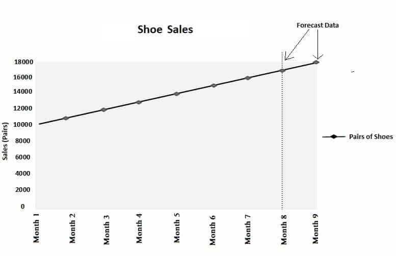
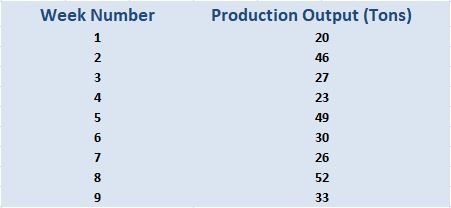
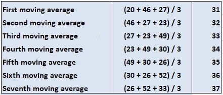
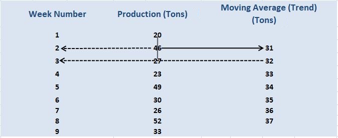
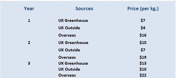
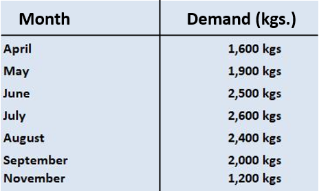
When preparing a cash budget (or the forecasts on which a cash budget is based), it is possible to use statistical techniques to arrive at valid estimates. Time series analysis is concerned with the numerical ways that the past can be used to forecast the future. The term trend analysis is also used to describe the technique examined in this article. It is useful as a tool to help forecast future sales, but it can also be used in other circumstances. In a nutshell, the idea of time series analysis is based on the assumption that in the future, data will continue to move in the same direction as they did in the past. Let's support the above-mentioned definition with an example. Suppose that a shoe manufacturer sells different numbers of pairs of shoes over a series of months. These data are shown as follows: Of course, this is a very simple example; life, on the other hand, is rarely this straightforward. It is also worth reflecting on the length of time for which this increase is likely to be sustainable. Before moving on, we'll examine useful techniques to forecast simple data. These basic techniques are essential for an understanding of the whole concept. In the above example, we can forecast future sales by noting that shoe sales increased by 1,000 every month. Using the last-known figure of 16,000 pairs of shoes in Month 7, we can simply add 1,000 to arrive at a forecast of 17,000 pairs in Month 8, and so on. A more complex technique can be used to arrive at the same answer. This technique is useful when each monthly change is different. Comparing the number of sales in Month 7 with the number in Month 1, there is an increase of 6,000 pairs. By dividing this figure by the number of times that the month changed in our data, we can arrive at an average change per month. The number of times that the month changes is 6, which is the same as the number of "spaces" between the months (or the total number of months minus 1). Shown as an equation, this becomes: Average monthly sales change = (Sales in final month - Sales in first month) / (Number of months - 1) = (16,000 - 10,000) / (7 - 1) = 1,000 (consistent with expectations) In turn, the figure of 1,000 can be added to the sales data of Month 7 (i.e., 16,000) to arrive at a forecast of 17,000 pairs of shoes sold in Month 8. The same result can be produced graphically. Using the same shoe shop as an example, we can extend the graph based on the actual data to form a forecast line. If the actual values do not change at a constant rate, using a graph will still produce the same answer provided that the straight-line runs through the first and last points. The data in the example can be expressed using the following formula: y = mx + c where To create a forecast for Month 8, the calculation is as follows: Forecast = (1,000 x number of months since Month 1) + 10,000 y (the forecast) = (1,000 x 7) + 10,000 = 17,000 (consistent with expectations) This formula works because it is based on a linear equation. In the above section, simple historical data was used to produce an estimate or forecast of future trends. To do this, the assumption was made that cyclical influences known as seasonal variations do not impact the data. Therefore, this section examines how historical data that may be influenced by regular cyclical variations can be used to generate a forecast. Moving averages are often useful to analyze historical data based on the following two main elements: The technique of moving averages demonstrated here can be used to generate the following types of data for cash budgets in certain circumstances: In all these situations, the technique will only provide valid data if the past movements in the data provide a good basis for a forecast of the future. A moving average is a term used to denote a series of averages calculated from a series of data (e.g., monthly sales or labor costs). In a moving average, the following two points apply: Suppose a manufacturing company's factory uses a manufacturing process that operates on a three-week cycle for technological reasons. At the end of each three-week period, the production vessels are cleaned and the process starts again. Meanwhile, as the factory workers become more adept at controlling the process, the output gradually increases. The production figures for the last few weeks are as follows: As the three-week cycle will influence the output, it is possible to calculate a three-point moving average as follows: An important point to notice is that we move along the list of data. In this simple example, which contains 9 pieces of data (one for each week), it is not possible to work out any more three-point averages. We have arrived at the end of the numbers after 7 calculations. Here, we chose the number of pieces of data to average each time so that it corresponded to the number of points in a full cycle (in this case, the three-week production cycle of the manufacturing business). By selecting three points corresponding to the number of weeks in the production cycle, we always had one example of the output of every type of week in our average. This means that any influence on the average by including the first week is canceled out due to the inclusion of data from a second and third week in the production cycle. We must, therefore, always be careful to calculate moving averages so that exactly one complete cycle is included in every average. Using moving averages, we have worked out the trend line. It is possible to use this to improve the sales forecast. A trend line is a line that shows a trend that can be plotted on a graph. When determining a trend line, each average relates to the data from its midpoint, as is shown in the layout of the figures we just calculated. This means that the first average we calculated (31 tons) can be used as the trend point of week 2, with the second point (32 tons) forming the trend point of week 3 (see dotted lines). The result is twofold: Even using our limited data in this example, we can see how to calculate seasonal variations. They are the difference between the actual data at a point and the trend at the same point. These seasonal variations are shown in the right-hand column of the table below. The data used are the features already calculated on the previous page. All the data are in tons. In this example, the seasonal variations repeat as follows: Note the way that plus and minus signs are used to denote the seasonal variations. You should be careful to calculate them accurately. Using the same data, production for future weeks can be calculated as follows: The forecasted production for Weeks 10-12 is carried out as follows: In this case, calculating the forecast trend is straightforward. This is because it consistently increases by 1 ton of output each week. This section shows how to use forecast data in a cash budget. Along with the information from the previous example, assume the following: The following receipts would appear in the cash budget for Weeks 12-16. Note that due to lagging, the receipts in Weeks 12 and 13 relate to the actual production in Weeks 8 and 9. The forecast data for Weeks 10-12 is used to calculate the receipts in Weeks 14-16. A case study is given below to demonstrate how the same technique can be used to forecast price data for a cash budget. A supermarket obtains supplies of the knawberry, a popular soft fruit, from three sources. The supplier used depends on the time of year, as indicated below. For the last three years, the prices that the supermarket has paid to suppliers are shown below. The monthly demand for the fruit, which will form the basis of the purchasing requirements, has already been calculated for the months of April—October of Year 4. These data are shown as follows: All growers are paid on two months' credit. Required: The trend in prices increases by $1 each season. We can use this with the seasonal variations to forecast the prices in Year 4. We can now use the demand data, together with the forecasted prices and credit period, to prepare the payments extract from the cash budget. It is worth noting that the amounts paid in June relate to April's purchases. This is because of the credit period. Hence, June's amounts are based on 1,600 kgs at $16. Similarly, the payments for July—October are based on overseas prices and quantities from May—August. The November payment is for overseas goods bought in September at $25 per kg.Time Series Analysis: Definition
Example
Month 1
10,000
Month 2
11,000
Month 3
12,000
Month 4
13,000
Month 5
14,000
Month 6
15,000
Month 7
16,000
Evidently, if the trend shown in the above table continues at the previous rate, then the company's shoe sales could be forecasted at 17,000 pairs in Month 8 and 18,000 pairs in Month 9.When Each Monthly Change Is Constant
Calculating the Change in Average Monthly Sales
Time Series Analysis: Graphs
Time Series Analysis: Formula
Time Series and Seasonal Variations
How Do Moving Averages Work?
Example
Finding the Trend Line
Calculating Seasonal Variations
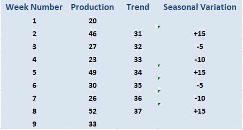

Using Forecast Data in the Cash Budget

Case Study: Forecasting Seasonal Prices
Situation
Solution
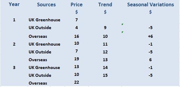


Time Series Analysis and Seasonal Variations FAQs
A time series is a set of data points collected at fixed time intervals.
Time series analysis can provide insights into a variety of business problems, including demand forecasting, trend identification and seasonality. It can also help to improve decision making by smoothing out fluctuations in a time series.
A moving average is an arithmetic mean that is calculated by adding the value of the current observation to the previous one and dividing the sum by two. The process continues until all observations have been utilized, at which point it starts again with the most recent observation.
Seasonal variations are changes that occur at fixed intervals and are due to predictable factors, such as the weather. They can impact demand, supply and price movements and need to be considered when forecasting prices.
A three-point moving average can be used to smooth out fluctuations in a time series and provide a more accurate forecast. It is calculated by adding the current observation to the previous two and dividing the sum by three. This process is then repeated for each new observation.
True Tamplin is a published author, public speaker, CEO of UpDigital, and founder of Finance Strategists.
True is a Certified Educator in Personal Finance (CEPF®), author of The Handy Financial Ratios Guide, a member of the Society for Advancing Business Editing and Writing, contributes to his financial education site, Finance Strategists, and has spoken to various financial communities such as the CFA Institute, as well as university students like his Alma mater, Biola University, where he received a bachelor of science in business and data analytics.
To learn more about True, visit his personal website or view his author profiles on Amazon, Nasdaq and Forbes.


