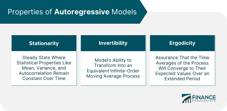
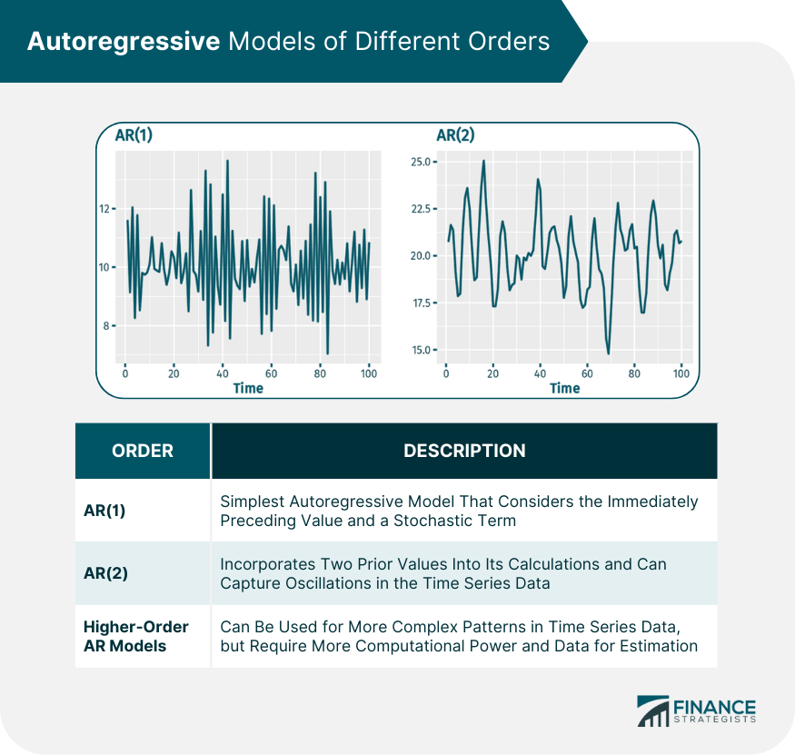
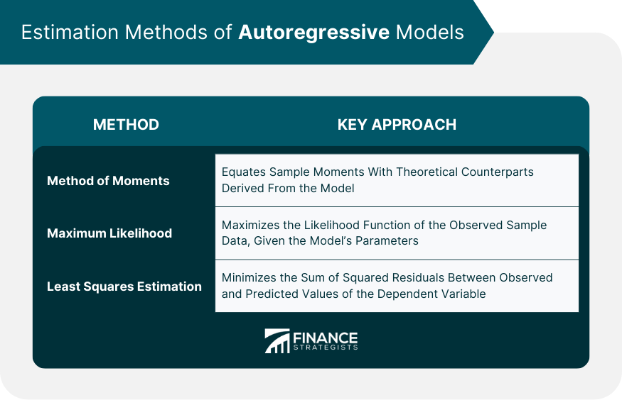
In the realm of statistics and econometrics, autoregressive models play an indispensable role, especially when it comes to time series analysis. As the name suggests, autoregressive models are statistical models where a variable's current value depends linearly on its own previous values. The term "autoregressive" means "self-regressive," implying that the present relies on the immediate past. The real-world applications of autoregressive models are extensive. From economic forecasting to financial market predictions, and even climate studies, they prove to be significant tools in interpreting past data to predict future values. By understanding the relationship of variables over time, analysts and researchers can make more informed decisions and forecasts. Key to the functionality of autoregressive models are three core properties: stationarity, invertibility, and ergodicity, each playing a significant role in the behavior and applicability of these models. In any autoregressive model, stationarity stands as a pivotal attribute. Stationarity essentially implies a steady state where statistical properties such as mean, variance, and autocorrelation persist unchanged over time. This property is essential for drawing reliable inferences from the model, as it ensures the consistency of patterns over time. To meet the criterion of stationarity in an AR(p) model, where 'p' denotes the order of the model, the roots of the model's characteristic equation must sit beyond the unit circle. This requirement ensures the model's stability, avoiding explosive behavior that could lead to unreliable predictions. The property of invertibility in an autoregressive model offers a unique perspective on the data at hand. An invertible model allows for transformation into an equivalent infinite-order moving average process. This transformation offers another way to interpret the data and can sometimes make the model easier to understand or estimate. It underscores the versatility and flexibility of autoregressive models, broadening their usability. Ergodicity is another key trait found in autoregressive models. It assures that over an extended time frame, the time averages of the process eventually converge to their expected values. This convergence occurs no matter the initial conditions of the process. The essence of ergodicity lies in its assurance that, given sufficient time, the model's outputs would represent the true underlying statistical properties of the process. This attribute is vital for validating long-term forecasts, as it provides an assurance of ultimate convergence towards actual values, despite potential short-term deviations. An AR(1) model, the simplest autoregressive model, describes a time series that evolves over time by considering the immediately preceding value and a stochastic term. The strength of dependence on the previous term is determined by a parameter known as the autoregressive coefficient. An AR(2) model incorporates two prior values into its calculations. This model can capture oscillations in the time series data, which the AR(1) model cannot. For more complex patterns in time series data, higher-order autoregressive models, such as AR(3), AR(4), etc., may be employed. However, these require more computational power and data for estimation. Three prominent estimation methods—Method of Moments, Maximum Likelihood Estimation, and Least Squares Estimation—serve this purpose, each with its unique approaches and benefits. This approach equates sample moments with their theoretical counterparts derived from the model. By solving the resulting system of equations, one can obtain estimates of the autoregressive coefficients. The simplicity and computational efficiency of the Method of Moments make it a popular choice in various applications. This technique focuses on maximizing the likelihood function of the observed sample data, given the model's parameters. By identifying the parameter values that yield the highest likelihood, MLE offers an optimized solution to estimate the autoregressive coefficients. MLE boasts desirable statistical properties, such as consistency and asymptotic normality, which make it an appealing choice for researchers and analysts. This, another widely-used technique, seeks to minimize the sum of squared residuals between the observed and predicted values of the dependent variable. By finding the autoregressive coefficients that yield the smallest sum of squared differences, LSE ensures that the model's predictions align closely with the actual data. This approach is relatively easy to implement and computationally efficient, making it a favorite among practitioners. Autoregressive models make several key assumptions: the data must be stationary, the relationship between variables and their lagged values must be linear, and the error term should be white noise. Despite their usefulness, autoregressive models can be subject to overfitting, incorrect model order selection, and assumptions not always held true, which may lead to inaccurate predictions. Autoregressive models are widely used in forecasting, from predicting stock prices to forecasting economic indicators like GDP, due to their ability to capture the evolution of statistical properties over time. Compared to other models like moving averages (MA), ARIMA, and state-space models, autoregressive models have their own strengths and weaknesses, making them more suitable for certain types of data and situations. By utilizing autoregressive models, analysts can evaluate past stock price trends to predict future movements, aiding in investment decisions. Autoregressive models serve a crucial role in economic forecasting. Economists use them to predict future economic conditions, including inflation rates, GDP growth, and unemployment rates. In risk management, autoregressive models help estimate potential losses and the likelihood of adverse events, assisting firms in mitigating potential threats. Autoregressive models, grounded in the statistical concept where current values of a variable are linearly dependent on their past counterparts, offer robust tools for understanding and forecasting trends in time series data. These models bear critical properties such as stationarity, invertibility, and ergodicity, which are fundamental for the models to function accurately and provide reliable predictions. The estimation of autoregressive models is achieved through various methods, including the Method of Moments, Maximum Likelihood Estimation, and Least Squares Estimation, all of which facilitate the computation of model parameters based on given data. Understanding these concepts and applying them to your financial strategies can significantly boost your wealth management efforts. Seek wealth management services to leverage these autoregressive models to deliver insights and make predictions that inform smart investment decisions. Definition of Autoregressive
Properties of Autoregressive Models
Stationarity
Invertibility
Ergodicity

Autoregressive Models of Different Orders
First-Order Autoregressive Model (AR(1))
Second-Order Autoregressive Model (AR(2))
Higher-Order Autoregressive Models

Estimation of Autoregressive Models
Method of Moments
Maximum Likelihood Estimation
Least Squares Estimation

Autoregressive Model Assumptions and Limitations
Assumptions for Validity
Potential Drawbacks and Misinterpretations
Autoregressive Models in Time Series Analysis
Use of Autoregressive Models in Forecasting
Comparisons With Other Time Series Models
Autoregressive Models in Financial Market Forecasting
Stock Market Analysis
Economic Forecasting
Risk Management
Bottom Line
Autoregressive FAQs
Autoregressive models are statistical models used in time series analysis where a variable's current value depends linearly on its own previous values.
Autoregressive models are significant in various fields, such as economics and finance, as they help forecast future values based on past data.
Common applications include economic forecasting, financial market predictions, risk management, and climate studies.
Limitations include potential overfitting, incorrect model order selection, and the necessity for certain assumptions (like stationarity and linear relationships) to hold.
Methods for estimating autoregressive models include the Method of Moments, Maximum Likelihood Estimation, and Least Squares Estimation.
True Tamplin is a published author, public speaker, CEO of UpDigital, and founder of Finance Strategists.
True is a Certified Educator in Personal Finance (CEPF®), author of The Handy Financial Ratios Guide, a member of the Society for Advancing Business Editing and Writing, contributes to his financial education site, Finance Strategists, and has spoken to various financial communities such as the CFA Institute, as well as university students like his Alma mater, Biola University, where he received a bachelor of science in business and data analytics.
To learn more about True, visit his personal website or view his author profiles on Amazon, Nasdaq and Forbes.


