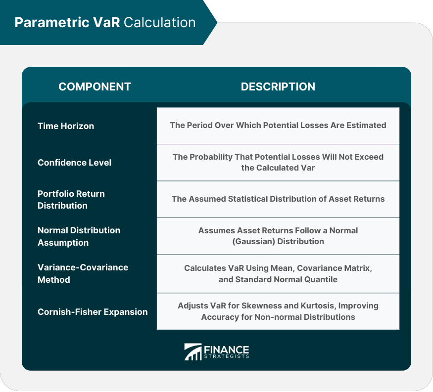
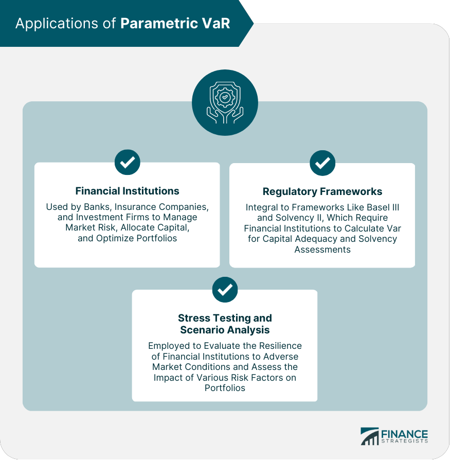
Parametric VaR, also known as the analytical VaR or variance-covariance VaR, is a method that relies on the statistical characteristics of asset returns, such as mean and standard deviation, to estimate potential losses. This approach assumes that asset returns follow a specific distribution, usually normal or Gaussian distribution. Two other popular VaR methods are Historical Simulation and Monte Carlo Simulation. Historical Simulation uses historical asset return data to calculate VaR, while Monte Carlo Simulation generates random scenarios based on predefined statistical characteristics. Parametric VaR is often preferred for its simplicity and speed, but its reliance on distributional assumptions can also be a limitation. Parametric VaR relies on several assumptions, including the normality of asset returns, linearity of portfolio returns, and the stability of risk factors over time. These assumptions may not hold true in practice, leading to inaccurate VaR estimations. Moreover, this method might not capture extreme events or non-linear relationships between assets effectively. Three essential components determine the calculation of parametric VaR: 1. Time Horizon: The period over which potential losses are estimated. 2. Confidence Level: The probability that the potential losses will not exceed the calculated VaR. 3. Portfolio Return Distribution: The assumed statistical distribution of asset returns. Parametric VaR typically assumes that asset returns follow a normal distribution, characterized by a bell-shaped curve. This assumption simplifies the calculation process, as only the mean and standard deviation of asset returns are required. However, the normality assumption is often criticized for underestimating extreme events and tail risks, as real-world financial data often exhibit fat-tailed distributions, skewness, and kurtosis. The variance-covariance method is the most common approach to calculating parametric VaR. The steps involved are: 1. Estimate the mean and covariance matrix of asset returns. 2. Determine the portfolio's expected return and standard deviation. 3. Calculate the VaR using the inverse of the standard normal distribution function, the portfolio's standard deviation, and the chosen confidence level. The variance-covariance method is computationally efficient and easy to implement. However, its accuracy depends on the validity of the normality assumption and the stability of the covariance matrix. Skewness and kurtosis are measures of a distribution's asymmetry and tail heaviness, respectively. The Cornish-Fisher expansion is a technique that adjusts the parametric VaR for these characteristics, improving its accuracy for non-normal distributions. The Cornish-Fisher expansion modifies the standard normal quantile used in the variance-covariance method by incorporating the skewness and kurtosis of asset returns. This adjustment results in a more accurate VaR estimate when the normality assumption does not hold. The Cornish-Fisher expansion provides a more robust VaR estimation for non-normal distributions. However, it requires more extensive data and additional calculations, making it less computationally efficient than the variance-covariance method. Parametric VaR is employed across various financial institutions, including banks, insurance companies, and investment firms, to manage market risk, allocate capital, and optimize investment portfolios. Parametric VaR plays a significant role in regulatory frameworks, such as Basel III for banks and Solvency II for insurance companies. These frameworks require financial institutions to calculate VaR to determine capital adequacy and solvency ratios. Financial institutions also use parametric VaR in stress testing and scenario analysis to evaluate their resilience to adverse market conditions and assess the impact of various risk factors on their portfolios. Parametric VaR's reliance on the normality assumption has been a point of criticism, as financial markets often exhibit non-normal behavior. This limitation can lead to underestimation of potential losses and inadequate risk management. The inability of parametric VaR to accurately capture fat-tailed distributions and extreme events exposes financial institutions to unexpected losses, as witnessed during the 2008 financial crisis. Parametric VaR models may suffer from model risk due to errors in data, assumptions, or calculations. Regular model validation and backtesting are essential to ensure the accuracy and reliability of VaR estimates. Parametric VaR relies on the diversification benefits arising from the covariance matrix. However, these benefits may not always be realized in practice, as correlations between assets can change during market stress or extreme events. Extreme Value Theory (EVT) is a statistical approach that focuses on modeling the tails of distributions, providing better estimates of VaR in the presence of extreme events. EVT-based VaR models have gained popularity as an alternative to parametric VaR. Copulas offer a flexible approach to model the dependence structure between assets, allowing for more accurate VaR estimation in the presence of non-linear relationships and changing correlations. Recent advances in machine learning have led to the development of new VaR estimation techniques that can better capture complex relationships between assets and accommodate non-normal distributions. Parametric VaR is a widely-used risk management tool that calculates potential portfolio losses based on the statistical characteristics of asset returns. While it offers simplicity and computational efficiency, its reliance on the normality assumption and other limitations can lead to inaccurate estimations. Alternative methods, such as the Cornish-Fisher expansion, have been developed to address these limitations and improve VaR accuracy. Parametric VaR remains a critical component in risk management for financial institutions and regulatory frameworks. Recent advances in EVT, copulas, and machine learning provide promising enhancements and alternatives to traditional parametric VaR models, contributing to more robust and accurate risk management practices in the financial industry.Parametric VaR: An Overview
Concept and Background
Comparison With Other VaR Methods
Assumptions and Limitations
Parametric VaR Calculation

Key Components
Normal Distribution Assumption
Characteristics and Rationale
Limitations and Criticism
Variance-Covariance Method
Steps in the Calculation
Advantages and Disadvantages
Cornish-Fisher Expansion
Introduction to Skewness and Kurtosis
Adjusting for Non-Normality
Advantages and Disadvantages
Applications of Parametric VaR

Financial Institutions
Regulatory Frameworks
Stress Testing and Scenario Analysis
Parametric VaR Challenges and Criticisms
Issues With Normality Assumption
Fat-Tailed Distributions and Extreme Events
Model Risk and Validation
Diversification Benefits and Limitations
Recent Developments and Alternatives
EVT-Based VaR Models
Copula-Based VaR Models
Machine Learning Techniques in VaR Estimation
Conclusion
Parametric VaR FAQs
Parametric VaR is a risk management metric that estimates potential portfolio losses using statistical characteristics of asset returns, such as mean and standard deviation. It is important in risk management as it helps financial institutions assess market risk, allocate capital efficiently, and optimize investment portfolios.
Parametric VaR relies on the assumption that asset returns follow a specific distribution, usually normal or Gaussian, and estimates potential losses using their mean and standard deviation. In contrast, Historical Simulation uses historical data, and Monte Carlo Simulation generates random scenarios based on predefined statistical characteristics. Parametric VaR is preferred for its simplicity and speed but may have limitations due to its reliance on distributional assumptions.
The main limitations of Parametric VaR include its reliance on the normality assumption, which can underestimate extreme events and tail risks, and its inability to capture non-linear relationships between assets effectively. Additionally, the stability of risk factors over time may be questioned, affecting the accuracy of VaR estimations.
The Cornish-Fisher expansion adjusts Parametric VaR for skewness and kurtosis, which are measures of a distribution's asymmetry and tail heaviness. By incorporating these characteristics into the standard normal quantile used in the variance-covariance method, the Cornish-Fisher expansion provides a more accurate VaR estimate when the normality assumption does not hold.
Recent developments and alternatives to Parametric VaR include Extreme Value Theory (EVT)-based VaR models, which focus on modeling the tails of distributions; copula-based VaR models, which offer a flexible approach to model the dependence structure between assets; and machine learning techniques, which can better capture complex relationships between assets and accommodate non-normal distributions.
True Tamplin is a published author, public speaker, CEO of UpDigital, and founder of Finance Strategists.
True is a Certified Educator in Personal Finance (CEPF®), author of The Handy Financial Ratios Guide, a member of the Society for Advancing Business Editing and Writing, contributes to his financial education site, Finance Strategists, and has spoken to various financial communities such as the CFA Institute, as well as university students like his Alma mater, Biola University, where he received a bachelor of science in business and data analytics.
To learn more about True, visit his personal website or view his author profiles on Amazon, Nasdaq and Forbes.


